A robot arm that has been taught a pouring motion is not doing anything difficult. It repeats the same arc whether or not there is a cup underneath it. The interesting question is the one the seminar kept circling — what can the robot really do? — and the honest answer is: only as much as it can see.
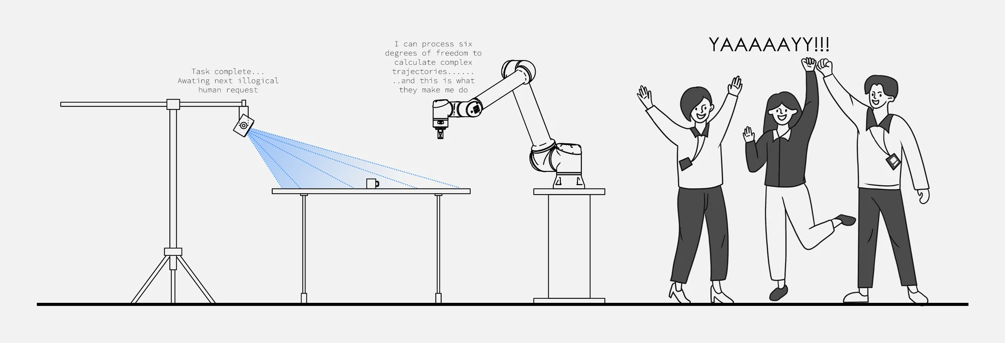
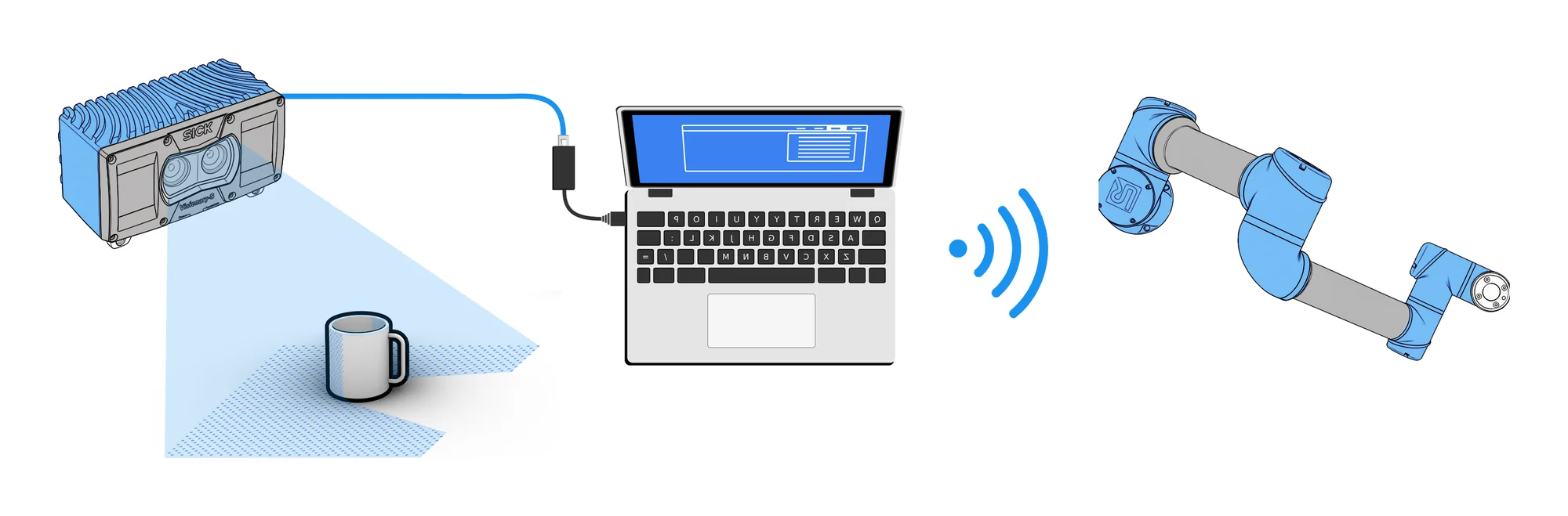
So the cup stopped being a coordinate. A SICK lidar sensor watches the table, and everything downstream is derived from what it finds there: where the cup is, how wide it is, how much it holds, and therefore how many seconds to keep pouring. Move the cup, re-scan, and every one of those numbers changes. Nothing about it is hard-coded.
- SICK SOPASEngineering tool · capture and filter
- PythonCoLa transport protocol · writes .ply
- Rhino + GrasshopperRobots plugin · trajectory and control
- Type
- Group project
- Team
- Hrithik Shetty, Bo Schneider
- My part
- Sensor pipeline and Grasshopper logic, jointly with Bo
- Seminar
- Collaborative Robotics in Architecture
- Supervision
- Victor Sardenberg, Ph.D.
- Location
- Detmold, Germany
- Course
- TH OWL — MID Computational Design
The trial that came first
Before the sensor was involved at all, the same arm learned to open a bottle and pour it into a mug at a position we typed in. That version taught us the constraint that shaped everything after it: each joint on the UR-10e only travels ±360°, so a cap that needs more than one full turn will run the wrist into its own limit mid-unscrew.
The fix is unglamorous and worth stating. The robot turns the cap 180° anticlockwise, lets go, lifts clear, rotates back clockwise to where it started, and takes a fresh grip. Threads longer than half a turn stop being a special case.
Stack
- SICK Visionary-S CX
- SOPAS Engineering Tool
- CoLa protocol
- Point clouds (.ply)
- Robots plugin
- UR-10e
Teaching it to look
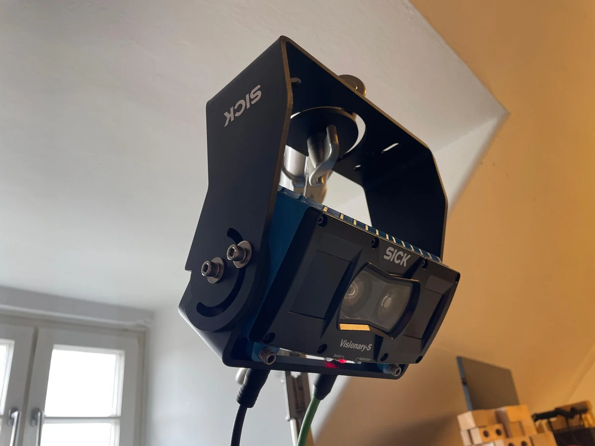
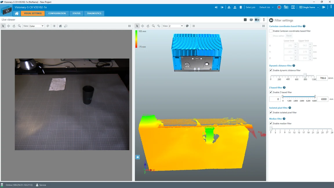
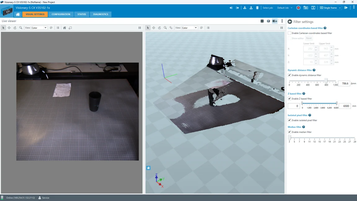
The sensor is a SICK Visionary-S CX on a stand above the table. Its own software, the SOPAS Engineering Tool, is where the scan gets useful: a dynamic distance filter, a Z-based filter, an isolated-pixel filter and a median filter, tuned until the table, the paper and the room fall away and the cup is most of what survives.
That tuning matters more than it sounds. Those filters are saved onto the sensor itself, so the capture script that runs later inherits them and returns a cloud that is already mostly cup.
Hurdles
- ±360° joint limits
- Plane orientation
- Sensor-to-robot coordinates
- Constant pour rate
Getting the data out
The lidar streams over SICK’s native CoLa protocol, which Grasshopper cannot read. Building on the sick_visionary_samples package from SICK AG, the capture script opens a TCP control connection and a stream on port 2114, and sets the one number that shapes everything after it: ten seconds between captures.
Then it stays in a loop. Each pass triggers a single snapshot, reads the frame off the stream in millimetres, and turns its depth map into a point cloud — real-world coordinates rather than pixels.
The detail that makes the loop useful is the file name. Every capture overwrites the same world_coordinates.ply, so Grasshopper never has to be told which scan is newest — it re-reads one path and always gets the current table. Move the cup, wait one cycle, and the graph is already looking at it.
The wait is measured, not fixed. The time the capture itself took is subtracted from the interval, so a slow frame does not push every later one back, and the scans stay ten seconds apart.
Ctrl+C ends the loop and reports how many frames it took.
def runSnapshotsDemo(ip_address: str, device_type: str):
    cola_protocol, control_port, _ = get_device_config(device_type)
    transport_protocol = "TCP"
    streaming_port = 2114
    write_files = True
    capture_interval = 10.0 #The time between two picture/pointclouds taken
    # …
    try:
        frame_count = 0
        # …
        while True:
            start_time = time.time()
            frame_count += 1

            # Trigger a snapshot
            device_control.singleStep()
            if transport_protocol == "TCP":
                streaming_device.getFrame()
                # …
                whole_frame = streaming_device.frame
                sensor_data.read(whole_frame, convertToMM=True)
                # …
                if sensor_data.hasDepthMap:
                    # …
                    if write_files:
                        world_coordinates, dist_data = convertToPointCloud(sensor_data.depthmap.distance,
                                                                        sensor_data.depthmap.intensity,
                                                                        sensor_data.depthmap.confidence,
                                                                        sensor_data.cameraParams, sensor_data.xmlParser.stereo)
                        # …
                        #This overwrite the existing PLY
                        writePointCloudToPLY(os.path.join(
                            pcl_dir, "world_coordinates.ply"), world_coordinates)
                        # …

            # Calculate time to wait for next capture
            time_elapsed = time.time() - start_time
            time_to_wait = max(0, capture_interval - time_elapsed)
            print(f"Waiting {time_to_wait:.2f} seconds until next capture...")
            time.sleep(time_to_wait)

    except KeyboardInterrupt:
        print(f"\nCapture stopped after {frame_count} frames")
It is a small script and deliberately so. It captures and it writes; every decision about what the cloud means is left to the graph, where it can be seen and changed.
From a cloud to a number
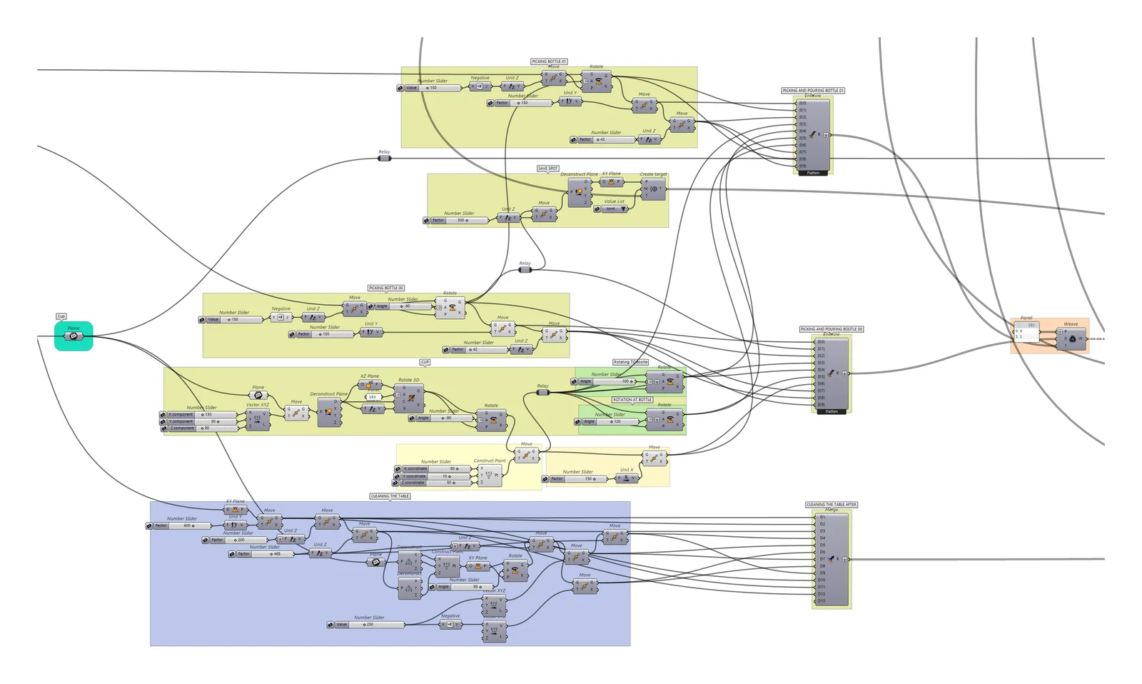
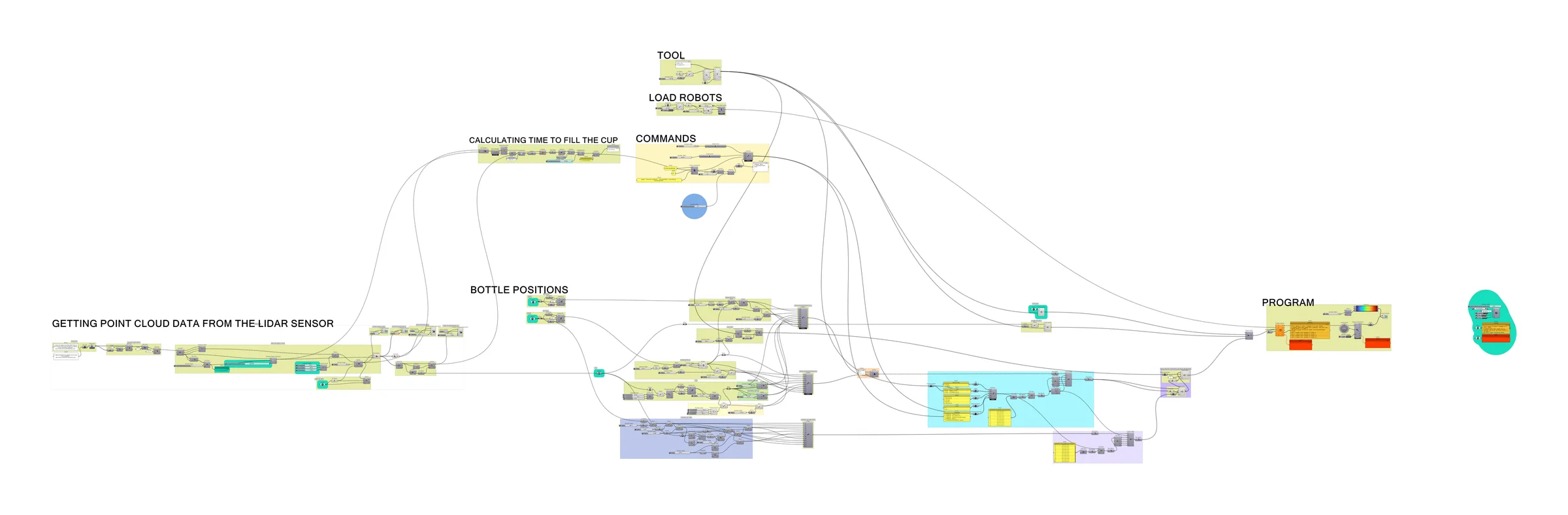
The graph opens the .ply, throws away everything that is not a point, and finds the highest Z value in what remains. A tolerance band below that height is kept, which isolates the rim of the cup rather than its sides, and a circle is fitted through it. That circle gives the cup’s centre and its radius in one move — the centre becomes the plane the robot pours at, the radius feeds the volume.
Fitting a circle rather than hunting for a centroid is the part worth keeping. A centroid drifts with whatever noise survives the filters; three points on a rim do not.
The pour is arithmetic
The rim circle is extruded down to the table, capped, and Grasshopper reports a volume. Multiply by a fill factor of 0.6 — nobody wants a glass filled to the brim — divide by the measured flow of the spout, and the answer is a number of seconds.
On the run captured here that came out at 35.67 seconds, from a flow of roughly 0.0153 litres per second and a table height of 797 mm. Change the cup and every one of those figures moves.

Two bottles, one cup
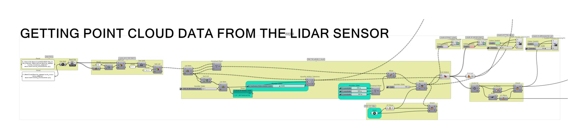
With a target plane and a duration, the rest is choreography: pick the first bottle, carry it to the cup, rotate it to the angle where liquid actually leaves the spout, hold for the calculated time, rotate back, return it, and repeat with the second. The tilt is its own small problem — pour too shallow and nothing comes out, too steep and the rate stops being constant, which breaks the arithmetic the whole thing rests on.
Then it wipes the table. A sponge is picked up and run over the drips, because a bartender that leaves a mess has not finished the job.
Robot control
- Gripper level
- Custom commands
- Wait / dwell
- Plane orientation
- Pick and place